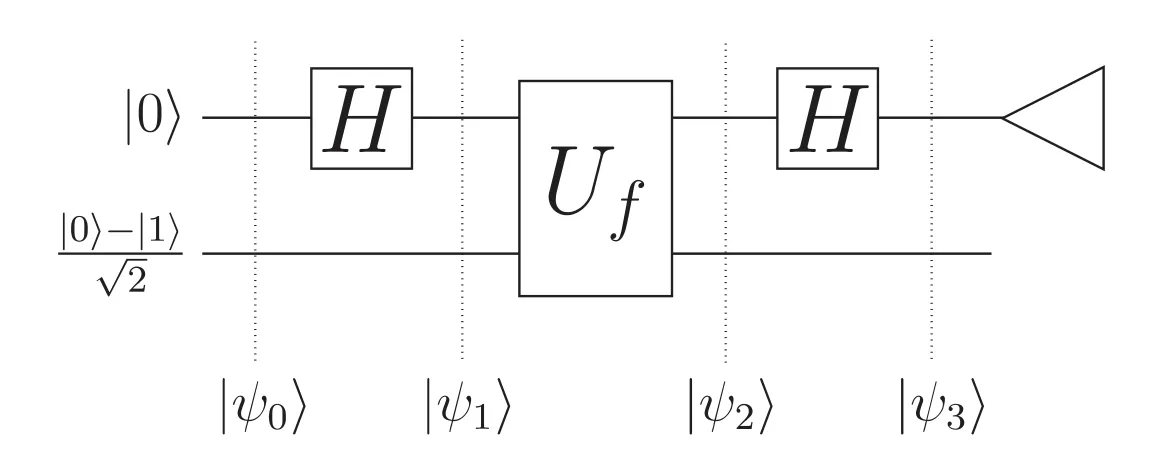
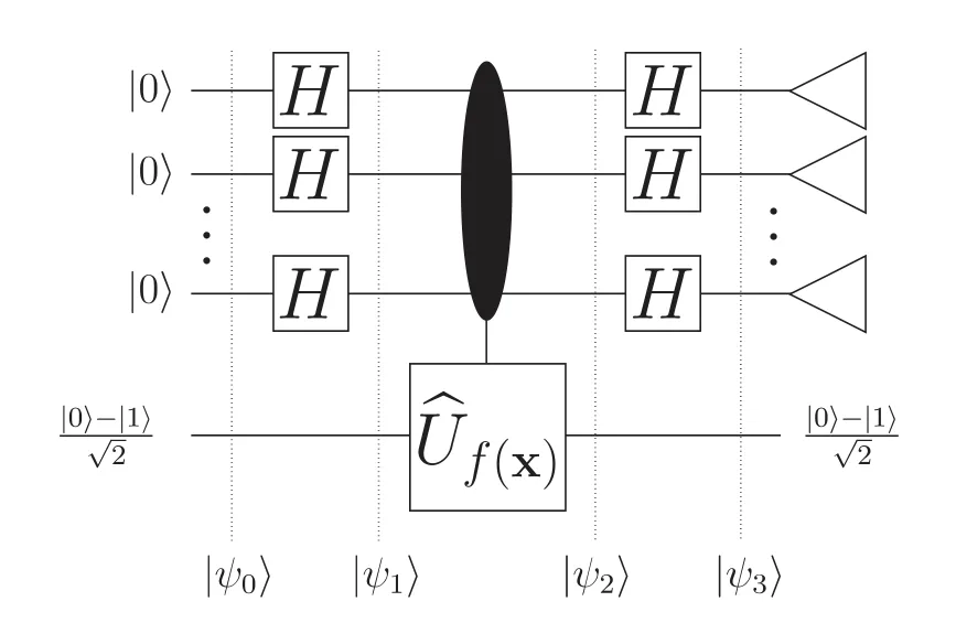
El algoritmo de Deutsch–Jozsa resuelve el problema que es una generalización del problema anterior. Ahora tenemos una función
f : { 0 , 1 } n → { 0 , 1 } f:\left\{ 0,1 \right\} ^{n} \rightarrow \left\{ 0,1 \right\} f : { 0 , 1 } n → { 0 , 1 } Aquí { 0 , 1 } n \left\{ 0,1 \right\}^{n} { 0 , 1 } n n n n
Es decir, si f ( x ) f(x) f ( x ) x x x f ( x ) = 0 f(x)=0 f ( x ) = 0 f ( x ) = 1 f(x)=1 f ( x ) = 1
Pensemos en el caso más simple, veamos qué pasa con el entero más pequeño que no sea 1.
f : { 0 , 1 } 2 → { 0 , 1 } f:\left\{ 0,1 \right\}^{2}\rightarrow \left\{ 0,1 \right\} f : { 0 , 1 } 2 → { 0 , 1 } Nuestras posibles entradas son { 00 } \left\{ 00 \right\} { 00 } { 01 } \left\{ 01 \right\} { 01 } { 10 } \left\{ 10 \right\} { 10 } { 11 } \left\{ 11 \right\} { 11 }
Observamos que tenemos 2 2 2^{2} 2 2 { 00 } \left\{ 00 \right\} { 00 } { 01 } \left\{ 01 \right\} { 01 } 0 0 0 1 1 1 (numero de mitad de entradas + 1) \text{(numero de mitad de entradas + 1)} (numero de mitad de entradas + 1)
De nuevo, tomando ventaja de la superposición cuántica y la interferencia, el algoritmo de Deutsch–Jozsa nos dice si f f f una única pregunta/evaluación.
Análogamente tendríamos que definir la operación cuántica:
U f : ∣ x ⟩ ∣ y ⟩ → ∣ x ⟩ ∣ y ⊕ f ( x ) ⟩ U_{f}:\ket{\mathbf{x}}\ket{y} \rightarrow \ket{\mathbf{x}}\ket{y \oplus f(x)} U f : ∣ x ⟩ ∣ y ⟩ → ∣ x ⟩ ∣ y ⊕ f ( x ) ⟩ donde x \mathbf{x} x n n n
Ahora, donde antes teníamos que:
Ahora tendremos:
Por lo tanto, empezamos en el estado
∣ ψ 0 ⟩ = ∣ 0 ⟩ ⊗ n ( ∣ 0 ⟩ − ∣ 1 ⟩ 2 ) \ket{\psi_{0}}=\ket{0} ^{\otimes n}\left( \frac{\ket{0}-\ket{1}}{\sqrt{ 2 }} \right) ∣ ψ 0 ⟩ = ∣ 0 ⟩ ⊗ n ( 2 ∣ 0 ⟩ − ∣ 1 ⟩ ) lo primero que tenemos que ver es qué pasa cuando hacemos H ⊗ n ∣ 0 ⟩ ⊗ n H^{\otimes n}\ket{0}^{\otimes n} H ⊗ n ∣ 0 ⟩ ⊗ n H ∣ 0 ⟩ = ∣ 0 ⟩ + ∣ 1 ⟩ 2 H\ket{0}=\frac{\ket{0}+\ket{1}}{\sqrt{ 2 }} H ∣ 0 ⟩ = 2 ∣ 0 ⟩ + ∣ 1 ⟩
H ⊗ 2 ∣ 0 ⟩ ⊗ 2 = H ∣ 0 ⟩ H ∣ 0 ⟩ = ( ∣ 0 ⟩ + ∣ 1 ⟩ 2 ) ⊗ ( ∣ 0 ⟩ + ∣ 1 ⟩ 2 ) = 1 2 ( ∣ 0 ⟩ + ∣ 1 ⟩ ) ⊗ ( ∣ 0 ⟩ + ∣ 1 ⟩ ) = 1 2 ( ∣ 00 ⟩ + ∣ 01 ⟩ + ∣ 10 ⟩ + ∣ 11 ⟩ ) \begin{aligned} H^{\otimes_{2}}\ket{0}^{\otimes_{2}} &= H\ket{0} H\ket{0} \\ &=\left( \frac{\ket{0}+\ket{1}}{\sqrt{ 2 }} \right)\otimes \left( \frac{\ket{0}+\ket{1}}{\sqrt{ 2 }} \right) \\ &= \frac{1}{2}(\ket{0}+\ket{1} )\otimes(\ket{0}+\ket{1} ) \\ &= \frac{1}{2}(\ket{00}+\ket{01}+\ket{10}+\ket{11} ) \end{aligned} H ⊗ 2 ∣ 0 ⟩ ⊗ 2 = H ∣ 0 ⟩ H ∣ 0 ⟩ = ( 2 ∣ 0 ⟩ + ∣ 1 ⟩ ) ⊗ ( 2 ∣ 0 ⟩ + ∣ 1 ⟩ ) = 2 1 ( ∣ 0 ⟩ + ∣ 1 ⟩ ) ⊗ ( ∣ 0 ⟩ + ∣ 1 ⟩ ) = 2 1 ( ∣ 00 ⟩ + ∣ 01 ⟩ + ∣ 10 ⟩ + ∣ 11 ⟩ ) como podemos ver, son todas las posibles combinaciones de dos bits.
Si n = 3 n=3 n = 3
H ∣ 0 ⟩ H ∣ 0 ⟩ H ∣ 0 ⟩ = 1 2 3 ( ∣ 0 ⟩ + ∣ 1 ⟩ ) ⊗ ( ∣ 0 ⟩ + ∣ 1 ⟩ ) ⊗ ( ∣ 0 ⟩ + ∣ 1 ⟩ ) H\ket{0}H\ket{0}H\ket{0} = \frac{1}{\sqrt{ 2^{3} }}(\ket{0}+\ket{1} )\otimes(\ket{0}+\ket{1} )\otimes(\ket{0}+\ket{1} ) H ∣ 0 ⟩ H ∣ 0 ⟩ H ∣ 0 ⟩ = 2 3 1 ( ∣ 0 ⟩ + ∣ 1 ⟩ ) ⊗ ( ∣ 0 ⟩ + ∣ 1 ⟩ ) ⊗ ( ∣ 0 ⟩ + ∣ 1 ⟩ ) Entonces, tendríamos algo así
H ⊗ n ∣ 0 ⟩ ⊗ n = H ∣ 0 ⟩ ⊗ ⋯ ⊗ H ∣ 0 ⟩ = 1 2 n ∑ x ∈ { 0 , 1 } n ∣ x ⟩ \begin{aligned} H^{\otimes n}\ket{0}^{\otimes n} &= H\ket{0} \otimes \dots \otimes H\ket{0} \\ &= \frac{1}{\sqrt{ 2^{n} }} \sum_{\mathbf{x}\in \left\{ 0,1 \right\}^{n} } \ket{\mathbf{x}} \end{aligned} H ⊗ n ∣ 0 ⟩ ⊗ n = H ∣ 0 ⟩ ⊗ ⋯ ⊗ H ∣ 0 ⟩ = 2 n 1 x ∈ { 0 , 1 } n ∑ ∣ x ⟩ Por lo tanto, el siguiente estado al estado inicial sería
∣ ψ 1 ⟩ = 1 2 n ∑ x ∈ { 0 , 1 } n ∣ x ⟩ ( ∣ 0 ⟩ − ∣ 1 ⟩ 2 ) \ket{\psi_{1}} = \frac{1}{\sqrt{ 2^{n} }}\sum_{\mathbf{x \in \left\{ 0,1 \right\}^{n} }} \ket{\mathbf{x}} \left( \frac{\ket{0}-\ket{1}}{\sqrt{ 2 }} \right) ∣ ψ 1 ⟩ = 2 n 1 x ∈ { 0 , 1 } n ∑ ∣ x ⟩ ( 2 ∣ 0 ⟩ − ∣ 1 ⟩ ) y siguiendo con el algoritmo, tendríamos que
∣ ψ 2 ⟩ = 1 2 n U f ( ∑ x ∈ { 0 , 1 } n ∣ x ⟩ ( ∣ 0 ⟩ − ∣ 1 ⟩ 2 ) ) \ket{\psi_{2}}= \frac{1}{\sqrt{ 2^{n} }}U_{f}\left( \sum_{\mathbf{x \in \left\{ 0,1 \right\}^{n} }} \ket{\mathbf{x}} \left( \frac{\ket{0}-\ket{1}}{\sqrt{ 2 }} \right) \right) ∣ ψ 2 ⟩ = 2 n 1 U f ⎝ ⎛ x ∈ { 0 , 1 } n ∑ ∣ x ⟩ ( 2 ∣ 0 ⟩ − ∣ 1 ⟩ ) ⎠ ⎞
En la entrada anterior se vio detenidamente que
U f : ∣ x ⟩ ( ∣ 0 ⟩ − ∣ 1 ⟩ 2 ) → ( − 1 ) f ( x ) ∣ x ⟩ ( ∣ 0 ⟩ − ∣ 1 ⟩ 2 ) U_{f}:\ket{x}\left( \frac{\ket{0}-\ket{1}}{\sqrt{ 2 }} \right) \rightarrow (-1)^{f(x)}\ket{x}\left( \frac{\ket{0}-\ket{1}}{\sqrt{ 2 }} \right) U f : ∣ x ⟩ ( 2 ∣ 0 ⟩ − ∣ 1 ⟩ ) → ( − 1 ) f ( x ) ∣ x ⟩ ( 2 ∣ 0 ⟩ − ∣ 1 ⟩ ) Por lo anterior, tenemos entonces
∣ ψ 2 ⟩ = 1 2 n ∑ x ∈ { 0 , 1 } n ( − 1 ) f ( x ) ∣ x ⟩ ( ∣ 0 ⟩ − ∣ 1 ⟩ 2 ) \ket{\psi_{2}} = \frac{1}{\sqrt{ 2^{n} }}\sum_{\mathbf{x \in \left\{ 0,1 \right\}^{n} }}(-1)^{f(\mathbf{x})}\ket{\mathbf{x}}\left( \frac{\ket{0}-\ket{1}}{\sqrt{ 2 }} \right) ∣ ψ 2 ⟩ = 2 n 1 x ∈ { 0 , 1 } n ∑ ( − 1 ) f ( x ) ∣ x ⟩ ( 2 ∣ 0 ⟩ − ∣ 1 ⟩ ) Ahora, tendríamos que aplicar H ⊗ n ∣ x ⟩ H^{\otimes n}\ket{\mathbf{x}} H ⊗ n ∣ x ⟩ ∣ x ⟩ \ket{x} ∣ x ⟩
H ∣ x ⟩ = 1 2 ( ∣ 0 ⟩ + ( − 1 ) x ∣ 1 ⟩ ) = 1 2 ∑ z ∈ { 0 , 1 } ( − 1 ) x z ∣ z ⟩ \begin{aligned} H\ket{x} &= \frac{1}{\sqrt{ 2 }}(\ket{0} + (-1)^{x}\ket{1} ) \\ &= \frac{1}{\sqrt{ 2 }}\sum_{z \in \left\{ 0,1 \right\} } (-1)^{xz}\ket{z} \end{aligned} H ∣ x ⟩ = 2 1 ( ∣ 0 ⟩ + ( − 1 ) x ∣ 1 ⟩ ) = 2 1 z ∈ { 0 , 1 } ∑ ( − 1 ) x z ∣ z ⟩ Entonces, tendríamos que (aquí se pone fea la cosa):
H ⊗ n ∣ x ⟩ = H ⊗ n ( ∣ x 1 ⟩ ∣ x 2 ⟩ … ∣ x n ⟩ ) = H ∣ x 1 ⟩ H ∣ x 2 ⟩ … H ∣ x n ⟩ = 1 2 ( ∣ 0 ⟩ + ( − 1 ) x 1 ∣ 1 ⟩ ) 1 2 ( ∣ 0 ⟩ + ( − 1 ) x 2 ∣ 1 ⟩ ) … 1 2 ( ∣ 0 ⟩ + ( − 1 ) x n ∣ 1 ⟩ ) = 1 2 ∑ z 1 ∈ { 0 , 1 } ( − 1 ) x 1 z 1 ∣ z 1 ⟩ 1 2 ∑ z 2 ∈ { 0 , 1 } ( − 1 ) x 2 z 2 ∣ z 2 ⟩ … 1 2 ∑ z n ∈ { 0 , 1 } ( − 1 ) x n z n ∣ z n ⟩ = 1 2 n ∑ z 1 z 2 … z n ∈ { 0 , 1 } n ( − 1 ) x 1 z 1 + x 2 z 2 + ⋯ + x n z n ∣ z 1 ⟩ ∣ z 2 ⟩ … ∣ z n ⟩ = 1 2 n ∑ z ∈ { 0 , 1 } n ( − 1 ) x ⋅ z ∣ z ⟩ \begin{aligned} H^{\otimes n}\ket{\mathbf{x}}&=H^{\otimes n}(\ket{x_{1}}\ket{x_{2}}\dots \ket{x_{n}} ) \\ &= H\ket{x_{1}}H\ket{x_{2}}\dots H\ket{x_{n}} \\ &= \frac{1}{\sqrt{ 2 }}(\ket{0} + (-1)^{x_{1}}\ket{1} )\frac{1}{\sqrt{ 2 }}(\ket{0} + (-1)^{x_{2}}\ket{1} )\dots\frac{1}{\sqrt{ 2 }}(\ket{0} + (-1)^{x_{n}}\ket{1} ) \\ &=\frac{1}{\sqrt{ 2 }}\sum_{z_{1} \in \left\{ 0,1 \right\} } (-1)^{x_{1}z_{1}}\ket{z_{1}} \frac{1}{\sqrt{ 2 }}\sum_{z_{2} \in \left\{ 0,1 \right\} } (-1)^{x_{2}z_{2}}\ket{z_{2}}\dots \frac{1}{\sqrt{ 2 }}\sum_{z_{n} \in \left\{ 0,1 \right\} } (-1)^{x_{n}z_{n}}\ket{z_{n}} \\ &=\frac{1}{\sqrt{ 2^{n} }}\sum_{z_{1}z_{2}\dots z_{n}\in \left\{ 0,1 \right\} ^{n}}(-1)^{x_{1}z_{1}+x_{2}z_{2}+\dots+x_{n}z_{n}}\ket{z_{1}} \ket{z_{2}} \dots \ket{z_{n}} \\ &= \frac{1}{\sqrt{ 2^{n} }}\sum_{\mathbf{z}\in \left\{ 0,1 \right\}^{n} }(-1)^{\mathbf{x}\cdot \mathbf{z}}\ket{\mathbf{z}} \end{aligned} H ⊗ n ∣ x ⟩ = H ⊗ n ( ∣ x 1 ⟩ ∣ x 2 ⟩ … ∣ x n ⟩ ) = H ∣ x 1 ⟩ H ∣ x 2 ⟩ … H ∣ x n ⟩ = 2 1 ( ∣ 0 ⟩ + ( − 1 ) x 1 ∣ 1 ⟩ ) 2 1 ( ∣ 0 ⟩ + ( − 1 ) x 2 ∣ 1 ⟩ ) … 2 1 ( ∣ 0 ⟩ + ( − 1 ) x n ∣ 1 ⟩ ) = 2 1 z 1 ∈ { 0 , 1 } ∑ ( − 1 ) x 1 z 1 ∣ z 1 ⟩ 2 1 z 2 ∈ { 0 , 1 } ∑ ( − 1 ) x 2 z 2 ∣ z 2 ⟩ … 2 1 z n ∈ { 0 , 1 } ∑ ( − 1 ) x n z n ∣ z n ⟩ = 2 n 1 z 1 z 2 … z n ∈ { 0 , 1 } n ∑ ( − 1 ) x 1 z 1 + x 2 z 2 + ⋯ + x n z n ∣ z 1 ⟩ ∣ z 2 ⟩ … ∣ z n ⟩ = 2 n 1 z ∈ { 0 , 1 } n ∑ ( − 1 ) x ⋅ z ∣ z ⟩ Por lo tanto, ahora sí ya sabemos que nuestro siguiente estado sería:
∣ ψ 3 ⟩ = ( 1 2 n ∑ x ∈ { 0 , 1 } n ( − 1 ) f ( x ) 1 2 n ∑ z ∈ { 0 , 1 } n ( − 1 ) x ⋅ z ∣ z ⟩ ) ( ∣ 0 ⟩ − ∣ 1 ⟩ 2 ) = 1 2 n ∑ z ∈ { 0 , 1 } n ( ∑ x ∈ { 0 , 1 } n ( − 1 ) f ( x ) + x ⋅ z ) ∣ z ⟩ ( ∣ 0 ⟩ − ∣ 1 ⟩ 2 ) \begin{aligned} \ket{\psi_{3}} &= \left( \frac{1}{\sqrt{ 2^{n} }}\sum_{\mathbf{x \in \left\{ 0,1 \right\}^{n} }}(-1)^{f(\mathbf{x})}\frac{1}{\sqrt{ 2^{n} }}\sum_{\mathbf{z}\in \left\{ 0,1 \right\}^{n} }(-1)^{\mathbf{x}\cdot \mathbf{z}}\ket{\mathbf{z}} \right) \left( \frac{\ket{0}-\ket{1}}{\sqrt{ 2 }} \right) \\ &= \frac{1}{2^{n}}\sum_{\mathbf{z}\in \left\{ 0, 1 \right\}^{n} }\left( \sum_{\mathbf{x \in \left\{ 0,1 \right\} ^{n}}}(-1)^{f(\mathbf{x})+\mathbf{x\cdot \mathbf{z}}} \right)\ket{\mathbf{z}}\left( \frac{\ket{0}-\ket{1}}{\sqrt{ 2 }} \right) \end{aligned} ∣ ψ 3 ⟩ = ⎝ ⎛ 2 n 1 x ∈ { 0 , 1 } n ∑ ( − 1 ) f ( x ) 2 n 1 z ∈ { 0 , 1 } n ∑ ( − 1 ) x ⋅ z ∣ z ⟩ ⎠ ⎞ ( 2 ∣ 0 ⟩ − ∣ 1 ⟩ ) = 2 n 1 z ∈ { 0 , 1 } n ∑ ⎝ ⎛ x ∈ { 0 , 1 } n ∑ ( − 1 ) f ( x ) + x ⋅ z ⎠ ⎞ ∣ z ⟩ ( 2 ∣ 0 ⟩ − ∣ 1 ⟩ ) Ahora, nuestro objetivo es analizar la amplitud asociada a cada estado base ∣ z ⟩ \ket{\mathbf{z}} ∣ z ⟩ f f f
La amplitud asociada a cada ∣ z ⟩ \ket{\mathbf{z}} ∣ z ⟩
A ( z ) = ∑ x ∈ { 0 , 1 } n ( − 1 ) f ( x ) + x ⋅ z A(\mathbf{z}) = \sum_{\mathbf{x} \in \{0,1\}^n} (-1)^{f(\mathbf{x}) + \mathbf{x} \cdot \mathbf{z}} A ( z ) = x ∈ { 0 , 1 } n ∑ ( − 1 ) f ( x ) + x ⋅ z Observamos que podemos separar el exponente:
( − 1 ) f ( x ) + x ⋅ z = ( − 1 ) f ( x ) ⋅ ( − 1 ) x ⋅ z (-1)^{f(\mathbf{x}) + \mathbf{x} \cdot \mathbf{z}} = (-1)^{f(\mathbf{x})} \cdot (-1)^{\mathbf{x} \cdot \mathbf{z}} ( − 1 ) f ( x ) + x ⋅ z = ( − 1 ) f ( x ) ⋅ ( − 1 ) x ⋅ z Por lo tanto, la amplitud es:
A ( z ) = ∑ x ( − 1 ) f ( x ) ( − 1 ) x ⋅ z A(\mathbf{z}) = \sum_{\mathbf{x}} (-1)^{f(\mathbf{x})} (-1)^{\mathbf{x} \cdot \mathbf{z}} A ( z ) = x ∑ ( − 1 ) f ( x ) ( − 1 ) x ⋅ z Si f ( x ) = 0 f(\mathbf{x}) = 0 f ( x ) = 0 x \mathbf{x} x
Entonces, ( − 1 ) f ( x ) = ( − 1 ) 0 = 1 (-1)^{f(\mathbf{x})} = (-1)^0 = 1 ( − 1 ) f ( x ) = ( − 1 ) 0 = 1
La amplitud se convierte en:
A ( z ) = ∑ x 1 ⋅ ( − 1 ) x ⋅ z = ∑ x ( − 1 ) x ⋅ z A(\mathbf{z}) = \sum_{\mathbf{x}} 1 \cdot (-1)^{\mathbf{x} \cdot \mathbf{z}} = \sum_{\mathbf{x}} (-1)^{\mathbf{x} \cdot \mathbf{z}} A ( z ) = x ∑ 1 ⋅ ( − 1 ) x ⋅ z = x ∑ ( − 1 ) x ⋅ z Sabemos que:
∑ x ( − 1 ) x ⋅ 0 = ∑ x 1 = 2 n \sum_{\mathbf{x}} (-1)^{\mathbf{x} \cdot \mathbf{0}} = \sum_{\mathbf{x}} 1 = 2^n x ∑ ( − 1 ) x ⋅ 0 = x ∑ 1 = 2 n ∑ x ( − 1 ) x ⋅ z = 0 \sum_{\mathbf{x}} (-1)^{\mathbf{x} \cdot \mathbf{z}} = 0 x ∑ ( − 1 ) x ⋅ z = 0 Por lo tanto, la amplitud es:
A ( z ) = { 2 n si z = 0 0 si z ≠ 0 A(\mathbf{z}) = \begin{cases} 2^n & \text{si } \mathbf{z} = \mathbf{0} \\ 0 & \text{si } \mathbf{z} \neq \mathbf{0} \end{cases} A ( z ) = { 2 n 0 si z = 0 si z = 0 Si f ( x ) = 1 f(\mathbf{x}) = 1 f ( x ) = 1 x \mathbf{x} x
Entonces, ( − 1 ) f ( x ) = ( − 1 ) 1 = − 1 (-1)^{f(\mathbf{x})} = (-1)^1 = -1 ( − 1 ) f ( x ) = ( − 1 ) 1 = − 1
La amplitud se convierte en:
A ( z ) = − ∑ x ( − 1 ) x ⋅ z A(\mathbf{z}) = -\sum_{\mathbf{x}} (-1)^{\mathbf{x} \cdot \mathbf{z}} A ( z ) = − x ∑ ( − 1 ) x ⋅ z Siguiendo el mismo razonamiento:
A ( z ) = { − 2 n si z = 0 0 si z ≠ 0 A(\mathbf{z}) = \begin{cases} -2^n & \text{si } \mathbf{z} = \mathbf{0} \\ 0 & \text{si } \mathbf{z} \neq \mathbf{0} \end{cases} A ( z ) = { − 2 n 0 si z = 0 si z = 0 Entonces en ambos casos, la única amplitud no nula es para z = 0 \mathbf{z} = \mathbf{0} z = 0 ∣ 0 ⟩ \ket{\mathbf{0}} ∣ 0 ⟩ n n n f f f
Para una función balanceada, hay un número igual de entradas donde f ( x ) = 0 f(\mathbf{x}) = 0 f ( x ) = 0 f ( x ) = 1 f(\mathbf{x}) = 1 f ( x ) = 1
Dividimos la suma en dos partes:
A ( z ) = ∑ x : f ( x ) = 0 ( − 1 ) 0 ( − 1 ) x ⋅ z + ∑ x : f ( x ) = 1 ( − 1 ) 1 ( − 1 ) x ⋅ z = S 0 − S 1 A(\mathbf{z}) = \sum_{\mathbf{x}: f(\mathbf{x})=0} (-1)^{0} (-1)^{\mathbf{x} \cdot \mathbf{z}} + \sum_{\mathbf{x}: f(\mathbf{x})=1} (-1)^{1} (-1)^{\mathbf{x} \cdot \mathbf{z}} = S_0 - S_1 A ( z ) = x : f ( x ) = 0 ∑ ( − 1 ) 0 ( − 1 ) x ⋅ z + x : f ( x ) = 1 ∑ ( − 1 ) 1 ( − 1 ) x ⋅ z = S 0 − S 1 Donde:
S 0 = ∑ x : f ( x ) = 0 ( − 1 ) x ⋅ z S_0 = \sum_{\mathbf{x}: f(\mathbf{x})=0} (-1)^{\mathbf{x} \cdot \mathbf{z}} S 0 = ∑ x : f ( x ) = 0 ( − 1 ) x ⋅ z
S 1 = ∑ x : f ( x ) = 1 ( − 1 ) x ⋅ z S_1 = \sum_{\mathbf{x}: f(\mathbf{x})=1} (-1)^{\mathbf{x} \cdot \mathbf{z}} S 1 = ∑ x : f ( x ) = 1 ( − 1 ) x ⋅ z
Como f f f
Sabemos que:
S 0 + S 1 = 2 n ⟹ S 0 = S 1 = 2 n − 1 S_0 + S_1 = 2^{n} \implies S_0 = S_1 = 2^{n-1} S 0 + S 1 = 2 n ⟹ S 0 = S 1 = 2 n − 1 Entonces, A ( 0 ) = S 0 − S 1 = 0 A(\mathbf{0}) = S_0 - S_1 = 0 A ( 0 ) = S 0 − S 1 = 0
S 0 + S 1 = 0 ⟹ S 0 = − S 1 S_0 + S_1 = 0 \implies S_0 = -S_1 S 0 + S 1 = 0 ⟹ S 0 = − S 1 Entonces, A ( z ) = S 0 − S 1 = 2 S 0 A(\mathbf{z}) = S_0 - S_1 = 2S_0 A ( z ) = S 0 − S 1 = 2 S 0
Sin embargo, dado que los valores de ( − 1 ) x ⋅ z (-1)^{\mathbf{x} \cdot \mathbf{z}} ( − 1 ) x ⋅ z + 1 +1 + 1 − 1 -1 − 1 S 0 S_0 S 0
Por lo que las amplitudes A ( z ) A(\mathbf{z}) A ( z ) z = 0 \mathbf{z} = \mathbf{0} z = 0 z ≠ 0 \mathbf{z} \neq \mathbf{0} z = 0 ∣ 0 ⟩ \ket{\mathbf{0}} ∣ 0 ⟩ n n n f f f
Después de la medición:
Si obtenemos z = 0 \mathbf{z} = \mathbf{0} z = 0 n n n , concluimos que f f f constante .
Si obtenemos cualquier otro valor de z \mathbf{z} z 0 \mathbf{0} 0 , concluimos que f f f balanceada .